Having represented this site as a technology blog with a focus on programming and software development, I find myself starting off with a tutorial on Excel basics instead. Somehow, I thought it was going to be more glamorous than this . . . This is driven by my need to prepare a training for my staff at work, and in keeping with the DRY principle (Don’t Repeat Yourself) I am killing two birds with one stone. Anyone hoping to read programming stuff is just going to have to wait . . .
Spreadsheets are misunderstood by the majority of people who use them. For many people a spreadsheet is nothing more than a handy way to create and organize lists. Some people use spreadsheets to present and layout data in a pleasing grid-like manner, and to apply pretty colors and formatting. If you are one of these people, you are missing out, and most likely working much harder than you need to.
Microsoft Excel, and other spreadsheets, are powerful data analysis tools. First and foremost, they are purpose-built to crunch numbers, twist, and manipulate information. A properly set up spreadsheet can make fast work out of calculations which would be laborious a few decades ago. While not really intended for this purpose, a spreadsheet can also serve as a small ad hoc database if no better alternative is available.
For even the most casual of users, properly understanding how a spreadsheet works, and how it handles the information you put into it will provide an almost immediate payoff. You do not have to be a “computer whiz” to get impressive results. Most importantly, you can save yourself time and pain by letting the spreadsheet do the heavy lifting for you. But before you can do that effectively, it is important to understand how Excel stores and works with information.
What’s an Expression?
Cells in a Microsoft Excel Spreadsheet may contain data, or they might contain an expression. Data is a value you type or otherwise place into a cell, such as Text, Numbers, Etc. (See Previous post in this series, Microsoft Excel Basics Part II: Data Types in Excel). The cell represents the actual value entered (despite any formatting which may cause it to display differently).
An expression is a statement or formula which returns a value. Further, an expression or formula might contain variables, meaning that the value returned by the expression might change depending upon the values provided as variables. If this is a little foggy for you, I will do my best to clarify in a minute. The point here is that, while within the cell, the formula is evaluated/computed what have you, from the spreadsheet perspective, the cell still represents a VALUE – the value returned by the formula.
While some of this becomes difficult to explain without creating even more confusion, expressions, formulas, and functions are what give Excel its real power. So this stuff is important to understand if you are to do anything with excel beyond keeping lists and laying out pages.
Here is an really simple example of a formula with one variable from every day life:
Let’s assume that you and a group of your friends are going to see a movie. Since you are the well-heeled benefactor of the group, you are paying for everyone’s movie ticket (If this is the type of person you are, shoot me an email – we should hang out. A lot.). The price of each movie ticket is $10.50 (yes, I really paid that much to go see a movie recently). How much will your total bill be?
Notice how you can’t quite answer that question yet? We know how much tickets cost (at THIS theater, anyway), but we don’t know how many of your friends are going yet, therefore we can’t know how much the total cost will be. However, we DO know that your final cost might be expressed as follows:
Total Cost = $10.50 X Number of Tickets Needed
In constructing the above (overly simple) formula, we determined the following:
- What we WANT to know (our desired output, if you will) is the Total Cost.
- What we already know is the cost per ticket.
- What we don’t know is the number of tickets we will be buying, which depends upon how many friends come to the movie with us.
Now, while everyone has different degrees of math aptitude, I will assume that, if you are reading this post, you would probably have mentally dealt with this, and performed the necessary computation in your head or with a calculator without breaking things down this far. But in essence, you have still mentally employed a formula.
Now let’s take our example a step further. Different theaters charge different prices for tickets. In fact, the same theater might charge a different price for a ticket depending on the time of day (the so-called matinee price). If we did not yet know where we planned to see the movie, we would introduce another unknown into our formula:
Total Cost = Ticket Price X Number of Tickets Needed
Now we have formula with TWO variables, Ticket Price and Number of Tickets Needed.
As we demonstrated in Part I of this series, we can use Microsoft Excel to perform simple calculations like this right in the cell. Let’s say we have determined that you will be taking 5 of your friends to see the matinee showing of Rise of the Planet of the Apes at a theater which charges $8.50 per ticket. You COULD do the following, which is kind of like using Excel as a calculator (remember to type the “equals” sign as the first part of any calculation or formula!):
| Before you hit Enter: | After you hit Enter: |
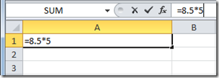 |
Note that we entered the value for Price per Ticket times the value of Number of Tickets Needed, just as our formula indicates. When we hit Enter, the result (the Total Cost) of 42.5 is displayed in the cell. For the purpose of Excel, the value displayed in the cell IS the Total Cost element in our formula above. This is all well and good for quick and dirty “one-off” calculations. But what if we wanted to be able to check the total cost for any number of friends, at any theater?
We can probably use Excel to come up with a more useful way of doing this. Let’s try this instead. We will create a Column Header for the Ticket Price,and another for Number of Tickets Needed. These can represent the variables in our formula. Then we will add a third column, Total Cost, which will represent the output of our formula. In THIS cell, we will re-write our formula using references to the values in the other cells:
| Before you hit Enter: | After you hit Enter: |
![Movie-Tix-Cell-Refs-Formula-Before-E[1] Movie-Tix-Cell-Refs-Formula-Before-E[1]](http://johnatten.com/wp-content/uploads/imported/Movie-Tix-Cell-Refs-Formula-Before-E%5B1%5D_thumb.png) |
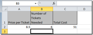
With THIS model, we can test different combinations of Price per Ticket and Number of Tickets Needed simply by typing new numerical values into the appropriate column. For example, if at the last minute your friend Jodi decided to go along, you would need six tickets instead of five. Simply enter the new value into the Number of Tickets Needed cell and hit enter:
| Before you hit Enter: | After you hit Enter: |
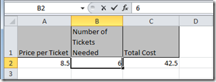 |
Voila! You now know that if the Number of Tickets Needed is six instead of five, the cost will be $51.00 instead of $42.50.
Your comfort level with creating your own formulas in Excel will depend to some degree upon your familiarity with basic algebra and other math. However, even if you have forgotten more math than you remember, it does not need to stop you from getting the most out of Excel. Some of the most commonly needed math operations are built in to Excel as functions.
What’s a Function?
A function is a bit like a formula, in that a function can use a combination of known values and variables, perform a calculation, and produce a result which can then be displayed, or used within OTHER functions or formulas. The difference between a formula and a function is that a function can be referenced by its name and will return the value of the calculation contained within. Confused yet?
Way back in the day, when I attended high school (up hill both ways, in the snow, etc. . . .), we were introduced to functions by way of the Function Machine. We will discuss that in a minute, but I am going to step out even further, because the function machine analogy was hard for me to grasp at first, simple though it is.
We’ll start with something a little more concrete. Let’s say you own a printer made by a particular manufacturer (say, Hewlett-Packard), which through bad luck or negligence, has ceased working properly. You decide you are going to get it repaired. You locate a printer repair shop which specializes in repairing HP printers, and which indicates the cost for repairs is a flat $50.00 (we’re keeping this simple).
What you want to do is drop your printer off, pay the man his $50.00, and leave with a working, repaired printer.
If we were to examine this situation from the perspective of a function machine, we might say that the printer repair shop is a Printer Repair Machine. You want to put your Broken Printer plus some money IN, and get back OUT a Working Printer. You are not real interested in what happens WITHIN the printer repair shop, how the man dissembles the printer, or what needs to be done to restore the printer to working order. What you want is a working printer.
We could break all that down like this:
The printer repair machine accepts input known as parameters or arguments, which must include a BROKEN PRINTER and $50.00. Upon receiving those inputs, the Printer Repair machine does one thing: PERFORM REPAIRS. When this action is complete, the printer repair machine provides the expected output, a WORKING PRINTER.
The printer repair machine itself is a bit like a black box. We don’t necessarily know what is going on when it does the PERFORM REPAIRS action, we just know that, barring any unexpected problems (or, error conditions), we can expect to receive a WORKING PRINTER when the printer repair machine is done.
About those unexpected problems. This carries a nice analogy as well. What if we brought in a broken bicycle instead? This might be regarded as an error. The shop would report that they cannot do the PERFORM REPAIR activity on a bicycle. Another example of unexpected problems might be if you only provided $40.00 instead of the required $50.00. In this case, the repair shop might kick out a message to you letting you know you have not provided enough money.
In the case above, we have a function Machine which performs a function: PERFORM REPAIRS. In order for PERFORM REPAIRS to execute properly, there are two required inputs, or parameters we need to supply: A BROKEN PRINTER, and MONEY ($50.00). If we put those two things into the Printer Repair Shop, the PERFORM REPAIR function is executed, and we receive a happy WORKING PRINTER as an output.
We could express this another way:
Working Printer = PERFORM REPAIRS(Broken Printer, Repair Fee)
In the above expression, the PERFORM REPAIRS function accepts the two required parameters and returns a Working Printer. In this syntax, the name of the function is used, followed by the parameter values, in a specific order, between the parentheses. The parameter values are separated by a comma.
Before I relate this back to functions in Excel, lets take things one step further. Let’s say that the printer repair shop will expedite the repair operation in under 24 hours for an additional fee of $10.00. Without the extra $10.00, the shop will only guarantee repairs within 5 working days. This is optional, for those customers who are in a hurry, and wish to pay a little extra to get the work done faster.
Now our diagram might look like this:
In THIS case, the PERFORM REPAIRS function requires at least the first two input parameters; a Broken Printer and $50.00. If the customer opts for the expedited repair option, the function will also accept an input of $10.00 and guarantee completion within 24 hours. Otherwise, the Working Printer output will be done in five working days.
In this case, we might use the following notation to express our function:
Working Printer = PERFORM REPAIRS(Broken Printer, Repair Fee, [Expedited Repair Fee])
In the above expression, the optional fee is notated in square brackets, indicating its optional status.
Excel Built-in Functions
SUM Some Values
Microsoft Excel has a plethora of built-in functions, in many different categories. To get us started, we will examine a few of those most commonly used for everyday spreadsheet tasks.
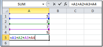
Not surprisingly, addition is probably THE most common thing we do in a spreadsheet. When we add the values represented by two or more cells, it can be tempting to write an expression like this:
Note that we are adding the values in the four cells above the current cell. However, there is a more efficient way to do this, using the built-in function SUM().
Remember, a function is a way to use a pre-defined formula or operation by using the name of the function, and providing any required (or sometime optional) parameters. In this case, the most basic function Excel provides us is called SUM, which, not surprisingly, returns the result of adding one or more numbers together.
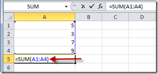
One way of using the SUM function is to provide a range of values as a parameter. It is no coincidence that I use the term range here. Remember from Part I of this series that a group of cells is also called a range? For example, in the example above, I am adding the values contained within the range of cells represented by cell A1 thru cell A4. Another way to write this is the range represented by A1:A4, where we separate the top left cell address and the bottom right cell address with a colon:
So in reality, our expression could be written like THIS:
| Before you hit Enter: | After you hit Enter: |
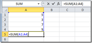 |
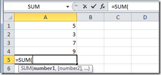
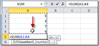
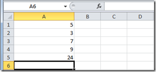
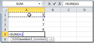
Wasn’t that a little more convenient? Also, note that while you CAN manually type the range into the cell, you can also use the following procedure, which can save a lot of time when you are doing a lot of “summing” over large ranges:
- Type the first part of the formula: =SUM(
- Use the mouse pointer to select the range you want to add by clicking on the first cell, and drag the mouse (while holding the mouse button down) across the range of cells to the last.
- When you let up the mouse button, the range you have selected will be surrounded by the “running ants” outline, and the address of the first and last cells of the range will be entered in your formula.
- Type the closing paren and hit enter.
| 1. Type Formula: | 2. Select First Cell: |
 |
| 3. Drag Down: | 4. Close Paren: |
 |
| 5. Hit Enter: | |
 |
It was harder to read through all those images than it was to make THAT formula happen, eh?
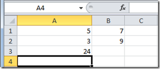
You can use the SUM function across any number of cells, within a single column or row, or spanning multiple columns and rows. For example, you could do THIS:
| Block Range (Before Enter): | Block Range (After Enter): |
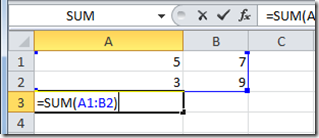 |
Note that in the above example, we told Excel to use the SUM function to add the values in the range A1:B2. The function correctly returned the value of 24.
As we learned previously, functions can use the results of other functions or calculations as input parameters as well. Let’s return to the sales order example from the first post in this series. We had created some column headings, and listed some items we might purchase, and quantities for each. Recall that we used a simple formula to calculate the total cost for the specified quantity of each item:
![Sales-Formula-Revisited---Showing-Fo[1] Sales-Formula-Revisited---Showing-Fo[1]](http://johnatten.com/wp-content/uploads/imported/Sales-Formula-Revisited---Showing-Fo%5B1%5D_thumb.png) Now we already know that we can use the SUM() function to add together the calculated item totals to arrive at a grand total for the order, because as we learned earlier, a formula or function can use the results of other formulas or functions as part of an additional calculation. So we could go ahead and type our SUM function into the cell just below the item totals to produce our grand total:
Now we already know that we can use the SUM() function to add together the calculated item totals to arrive at a grand total for the order, because as we learned earlier, a formula or function can use the results of other formulas or functions as part of an additional calculation. So we could go ahead and type our SUM function into the cell just below the item totals to produce our grand total:
Here is the same Sales Order example again, with the values displayed instead of formulas, and with the SUM() function typed into the appropriate cell:
| Sales Order Grand Total (Before Enter) | Sales Order Grand Total (After Enter) |
![Sales-Formula-Revisited---Grand-Tota[2] Sales-Formula-Revisited---Grand-Tota[2]](http://johnatten.com/wp-content/uploads/imported/Sales-Formula-Revisited---Grand-Tota%5B2%5D_thumb.png) |
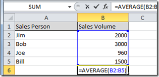
Another commonly used function which accepts a range as an input parameter is AVERAGE(). It does just what it sounds like – returns the average of a range of values. We type the name of the function, and then enclose the range we wish to average as a parameter within the parenthesis.
=AVERAGE(Some Range of Cells)
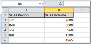
Let’s take a quick look at the average function. Let’s say that four salesmen have posted their stats for the quarter. We want to examine the average sales volume per sales person for statistical purposes. We could make a column named Sales Person and list each salesman’s name within that column. Then we could create a column Names Sales Volume in which we can list each salesman’s actual figure for the quarter. Then, using the AVERAGE() function, we can determine the average sales volume per sales person:
| Average Sales Volume (Before Enter): | Average Sales Volume (After Enter): |
 |
Ok. We have examined two commonly-used, but fairly rudimentary functions provided as part of Microsoft Excel’s built-in function set. In the next post, we will look at where to find an entire library of functions, and we will examine some more advanced functions and possible uses within a spreadsheet. After that, we will devote an entire post (or maybe two!) to formatting, and how formatting might affect what you see on screen as the result of certain functions.
Summary
- An expression is a formula or statement which returns a value.
- A function is a formula we refer to by name within an expression, which accepts parameters (sometimes called arguments) as input, and returns a value. The value of the output will be affected by the parameters provided as input(s).
- The SUM() Function can be used to add a range of values provided as an input parameter.
- The AVERAGE() function can be used to return the average of a range of values provided as an input parameter.
![Direct-Calculation-Movie-Tix-After-E[1] Direct-Calculation-Movie-Tix-After-E[1]](http://johnatten.com/wp-content/uploads/imported/Direct-Calculation-Movie-Tix-After-E%5B1%5D_thumb.png)
![Movie-Tix-Cell-Refs-Formula-After-En[1] Movie-Tix-Cell-Refs-Formula-After-En[1]](http://johnatten.com/wp-content/uploads/imported/Movie-Tix-Cell-Refs-Formula-After-En%5B1%5D_thumb.png)



![Sales-Formula-Revisited---Grand-Tota[4] Sales-Formula-Revisited---Grand-Tota[4]](http://johnatten.com/wp-content/uploads/imported/Sales-Formula-Revisited---Grand-Tota%5B4%5D_thumb.png)
Comments