Having represented this site as a technology blog with a focus on programming and software development, I find myself starting off with a tutorial on Excel basics instead. Somehow, I thought it was going to be more glamorous than this . . . This is driven by my need to prepare a training for my staff at work, and in keeping with the DRY principle (Don’t Repeat Yourself) I am killing two birds with one stone. Anyone hoping to read programming stuff is just going to have to wait . . .
If you do not have Microsoft Excel on you machine, or if you are using an older version (I use Excel 2010 throughout this series) you might consider purchasing a copy. You can find many deals on-line, or even support my efforts with this site by using the links above to buy directly from Microsoft. I STRONGLY recommend against purchasing software from Craigslist or EBay. There is significant risk of purchasing illegal or pirated software from those sites.
OK. If you have been following this little series, you are likely a beginning Excel User, or a glutton for punishment (or both). If you have not been following this series, but instead stumbled upon this entry, welcome to my series on Excel Basics.
We are going to step out of our examination of formulas and expressions for a moment to take a look at number formatting. While we touched on this subject very briefly in the first post, we will take a closer look now.
We will examine formatting from two perspectives. If you are an absolute beginner, you will learn how to apply formatting to cells, and a little about the various number formats themselves. If you are an intermediate or advanced user, you might find the section on the difference between the displayed format and the actual value stored in the cell to be a useful review.
For everyone’s benefit, let me put forth the following important reminder. Write this on your forehead:
It is the stored value that is used in calculations, NOT the displayed (formatted) value!
In this post
Formatting Basics (the VERY basics)
As we learned in the first post in this series, Microsoft Excel Basics Part II: Data Types in Excel, all number values (including dates) are stored by Excel a double-precision floating point values. How, then, do we know what is a date, what is currency, what is a percentage, and so on?
Formatting, that’s how.
Excel provides us with number formatting as a means to display a numerical value in a recognizable way relative to the context of use. If we are working with monetary values, it is helpful for our spreadsheet to display our data in a currency format. Likewise with dates and percentages. Exceptionally large (or exceptionally small) numerical values are often more effectively presented using scientific notation.
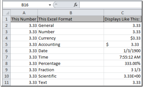
Let’s take a quick look at the basic number formats Microsoft Excel Provides. In the following image, the left-most column of cells all contain the same number value (3.33). The middle column describes the number format applied to the same value typed into the cells in the right-most column :
Applying Formatting
To apply formatting to a cell or group of cells, we right-click within the selected cell(s). Select the “Format Cells…” menu item from the context menu:
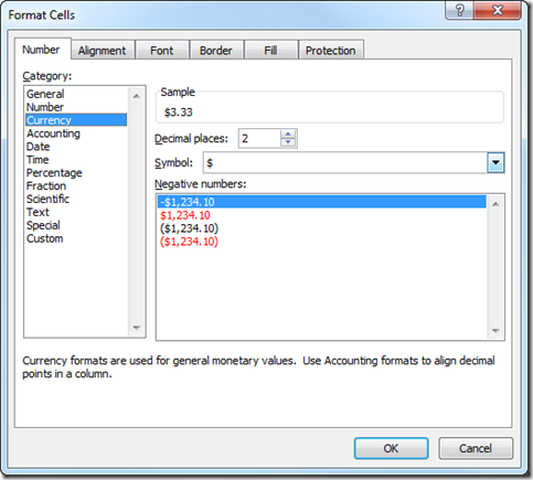
You will be presented with a dialog which allows you to select from a list of pre-defined number formats (plus a few special and user-defined ones). Selecting an item from the list of available formats on the left will cause various options for the selected format to become available in the space to the right of the list.
In this case, I am demonstrating the application of basic currency formatting. The options available for the currency format include number of decimal places, the desired currency symbol, and various means of representing negative numbers. The default values for all of these are what is displayed when you select the currency format (2 decimal places, US dollars (dependent upon your system localization settings) and the default representation for negative values. For this example, I am going with the defaults. When you hit the OK button, the 3.33 value we typed into the cell will be displayed as $3.33.
This is a good place to re-state the warning I posted in red at the beginning of this post:
It is the stored value that is used in calculations, NOT the displayed (formatted) value!
The hidden danger of number formatting in calculations
Open a new Excel Workbook. Then select the first two columns by clicking on the column headers (the gray rectangles with the letters A and B in them:
| Select column A: | Right-click and select “Format Cells” |
![Select Column A_thumb[9] Select Column A_thumb[9]](http://johnatten.com/wp-content/uploads/imported/Select%20Column%20A_thumb%5B9%5D_thumb.png) |
![Right Click Column A_thumb[8] Right Click Column A_thumb[8]](http://johnatten.com/wp-content/uploads/imported/Right%20Click%20Column%20A_thumb%5B8%5D_thumb.png) |
Now, do like we did in the first example, and format both columns as Currency. Use the default settings (2 decimal places, US currency, or whatever is native where you live). You will run into this format often in spreadsheet-land. Now select the first cell in column A (Cell A1), and type a simple formula to divide 10 by 3:
| Enter the formula: | Hit Enter: |
![Three Divided by Ten Before Enter Key_thumb[5] Three Divided by Ten Before Enter Key_thumb[5]](http://johnatten.com/wp-content/uploads/imported/Three%20Divided%20by%20Ten%20Before%20Enter%20Key_thumb%5B5%5D_thumb.png) |
![Three Divided by Ten After Enter Key_thumb[4] Three Divided by Ten After Enter Key_thumb[4]](http://johnatten.com/wp-content/uploads/imported/Three%20Divided%20by%20Ten%20After%20Enter%20Key_thumb%5B4%5D_thumb.png) |
Then, select the first cell in column B (Cell B1) and type the number 3.33:
| Enter the number 3.33: | Hit Enter: |
![Three Point Three Three Before Enter Key_thumb[1] Three Point Three Three Before Enter Key_thumb[1]](http://johnatten.com/wp-content/uploads/imported/Three%20Point%20Three%20Three%20Before%20Enter%20Key_thumb%5B1%5D_thumb.png) |
![Three Point Three Three After Enter Key_thumb[4] Three Point Three Three After Enter Key_thumb[4]](http://johnatten.com/wp-content/uploads/imported/Three%20Point%20Three%20Three%20After%20Enter%20Key_thumb%5B4%5D_thumb.png) |
Note that each cell now appears to contain the value of three dollars and thirty-three cents. Now we will use a logical test to illustrate why we need to be aware of how formatting can impact our spreadsheet design. We can compare the values stored in Cells A1 and B1 to see if they are equal. The following expression will return a logical result of TRUE or FALSE:
| Enter the formula =A=B | Hit Enter: |
![Compare A and B Before Enter_thumb[2] Compare A and B Before Enter_thumb[2]](http://johnatten.com/wp-content/uploads/imported/Compare%20A%20and%20B%20Before%20Enter_thumb%5B2%5D_thumb.png) |
![Compare A and B After Enter_thumb[1] Compare A and B After Enter_thumb[1]](http://johnatten.com/wp-content/uploads/imported/Compare%20A%20and%20B%20After%20Enter_thumb%5B1%5D_thumb.png) |
Now, why is that? I will say it one more time, for clarity:
It is the stored value that is used in calculations, NOT the displayed (formatted) value!
Excel treats the formula we entered into cell A1 as a value. The actual value of dividing the number ten by three is, in mathematical terms, 3.333333333333 . . . and so on. In performing the calculation, Excel carries this out to the limits of its 15 significant digits. While we see displayed $3.33, the value represented in the cell is actually 3.33333333333333. The number we entered into cell B1 is specifically 3.33.
Is 3.33 = 3.33333333333333?
No. The value in cell A1 is greater than the value in B1 by a little more than three one-thousandths. In other words, 3.33333333333333 > 3.33, and therefore, the expression testing whether or not the two values are equal returns FALSE.
A Side Note
If you select both columns again and remove the formatting (by setting the format back to “general”) you will see that the number in cell A1 is displayed as 3.3333333333, which is only 11 significant digits. However, if you select the cell and look in the formula bar, you will see all 15 significant digits. Again, what is displayed in the cell does not represent the exact value stored in the cell.
Be aware of numerical precision and rounding in ALL your formulas
When using Excel, it is important to bear in mind that number formatting can obscure the mathematical precision of values. This is especially true of calculations involving division, but can also apply to other operations as well. Most of the time, this will have little impact, particularly when dealing with currency values in the context of everyday business transactions.
However, in certain calculations, precision which is masked by formatting can introduce errors (usually rounding errors or comparison errors such as illustrated here) which might invalidate your worksheet. Equally as often, this type of error is not immediately apparent.
Formatting is our friend, and it present our data in a familiar context which makes for visually appealing spreadsheets. Best, however, to pay attention to results which appear not to make sense. There is likely a reason for that.
In another post, we will examine rounding and rounding errors, and how these can impact your spreadsheets.


Comments